Drawing 2D plots from FCS data in R with Bioconductor, base graphics and ggplot2

So I have spend the last few days working out how to generate nice 2D plots using flow cytometry data.

It's been interesting.

Here is the code and some nice output.


#load flowCore which allows the import of FCS files. 
source("http://bioconductor.org/biocLite.R")
biocLite("flowCore")
library(flowCore)

# import the data 
ntl<-read.FCS("A01 NTL.fcs", alter.names = TRUE)
n <- exprs(ntl)  # converts the data into a matrix
cd40L<-read.FCS("A02 CD40L.fcs", alter.names = TRUE)
c <- exprs(cd40L) # converts the data into a matrix

#BASE GRAPHICS
# Use base graphics of R to display FSC/SSC dot plots. 

par(mfrow=c(1,2)) #allows to plots to be placed side to side

plot(n[,1], n[,2], 
     pch = ".", 
     ylim=c(0,1000000),
     xlim=c(0,10000000),
     xlab="FSC-A",
     ylab="SSC-A",
     main="NTL") # this works

plot(c[,1], c[,2], 
     pch = ".", 
     ylim=c(0,1000000),
     xlim=c(0,10000000),
     xlab="FSC-A",
     ylab="SSC-A",
     main="CD40L") # this works

This is the plot produced:

#GGPLOT2
#Can also use ggplot2 to draw dot plots
library(ggplot2)

#seems ggplot only likes data frames
ndf <- as.data.frame(n) 
cdf <- as.data.frame(c)

#make the plotting objects using ggplot 
p1<- ggplot(ndf, aes(x=FSC.A, y=SSC.A)) + 
  geom_point(shape=".", colour="red") + 
  ylim(0, 500000) + xlim(0,5000000) +
  ggtitle("Samp 001, NTL & IL4")

p2<- ggplot(cdf, aes(x=FSC.A, y=SSC.A)) + 
  geom_point(shape=".", colour="red") + 
  ylim(0, 500000) + xlim(0,5000000) +
  ggtitle("Samp 001, CD40L & IL4")

multiplot(p1,p2, cols=2)

This is the output 

# 2D density plots
#with contour lines
p1 <- ggplot(ndf, aes(x=FSC.A, y=SSC.A)) + 
  geom_point(shape=".", colour="red") + 
  ylim(0, 500000) + xlim(0,5000000) +
  ggtitle("Samp 001, NTL & IL4") + 
  geom_density2d(colour="black", bins=5)

p2 <- ggplot(cdf, aes(x=FSC.A, y=SSC.A)) + 
  geom_point(shape=".", colour="red") + 
  ylim(0, 500000) + xlim(0,5000000) +
  ggtitle("Samp 001, NTL & IL4") + 
  geom_density2d(colour="black", bins=5)

multiplot(p1,p2, cols=2)

#with colour indicating density
ggplot(ndf, aes(x=FSC.A, y=SSC.A)) + 
  geom_point(shape=".", colour="red") + 
  ylim(0, 500000) + xlim(0,5000000) +
  ggtitle("Samp 001, NTL & IL4") + 
  stat_density2d(aes(alpha=..density..), geom="raster", contour = FALSE)

Some very useful help from here:
http://www.talkstats.com/showthread.php/52675-ggplot2-contour-chart-plotting-concentrations/page2

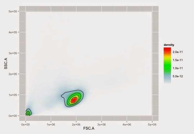
#with more colours indicating density
colfunc <- colorRampPalette(c("white", "lightblue", "green", "yellow", "red"))
ggplot(ndf, aes(x=FSC.A, y=SSC.A)) +
  ylim(0, 500000) + xlim(0,5000000) +
  stat_density2d(geom="tile", aes(fill = ..density..), contour = FALSE) +
  scale_fill_gradientn(colours=colfunc(400)) + 
  geom_density2d(colour="black", bins=5)

Cells on NTL with nice colours

ggplot(cdf, aes(x=FSC.A, y=SSC.A)) +
  ylim(0, 500000) + xlim(0,5000000) +
  stat_density2d(geom="tile", aes(fill = ..density..), contour = FALSE) +
  scale_fill_gradientn(colours=colfunc(400)) + 
  geom_density2d(colour="black", bins=5)

Cells on CD40L with nice colours

#function to allow more than one ggplot on a page
multiplot <- function(..., plotlist=NULL, file, cols=1, layout=NULL) {
  library(grid)
  
  # Make a list from the ... arguments and plotlist
  plots <- c(list(...), plotlist)
  
  numPlots = length(plots)
  
  # If layout is NULL, then use 'cols' to determine layout
  if (is.null(layout)) {
    # Make the panel
    # ncol: Number of columns of plots
    # nrow: Number of rows needed, calculated from # of cols
    layout <- matrix(seq(1, cols * ceiling(numPlots/cols)),
                     ncol = cols, nrow = ceiling(numPlots/cols))
  }
  
  if (numPlots==1) {
    print(plots[[1]])
    
  } else {
    # Set up the page
    grid.newpage()
    pushViewport(viewport(layout = grid.layout(nrow(layout), ncol(layout))))
    
    # Make each plot, in the correct location
    for (i in 1:numPlots) {
      # Get the i,j matrix positions of the regions that contain this subplot
      matchidx <- as.data.frame(which(layout == i, arr.ind = TRUE))
      
      print(plots[[i]], vp = viewport(layout.pos.row = matchidx$row,
                                      layout.pos.col = matchidx$col))
    }
  }
}